Multivariable Regression
1. Problem
Do modeling the performance of computer programs. The dataset provided describes a few examples of running SGDClassifier in Python. The features of the dataset describes the SGDClassifier as well as the features used to generate the synthetic training data. The data to be analyzed is the training time of the SGDClassifier.
Time is the training time of the model. The other feature follows the definition in Sklearn. Specifically, n_samples, n_features, n_classes, n_clusters_per_class, n_informative, flip_y, scale, describes how the synthetic dataset for training is generated using sklearn.datasets.make_classification, and penalty, l1_ratio, alpha, max_iter, random_state, n_jobs describes the setup of sklearn.linear_model.SGDClassifier
2. Solution
I analyse the relation between features in training data and do feature engineering for the better prediction. A feed forward neural network is used to predict running time.
2.1 Data Analysis
I analyse dataset in terms of the description in SGDClassifier in Scikit-Learn and use Numpy and Pandas.
train = pd.read_csv('../data/train.csv')
print('Shape of the train data with all features:', train.shape)

test = pd.read_csv('../data/test.csv')
print('Shape of the test data with all features:', test.shape)
Shape of the train data with all features: (400, 15)
Shape of the test data with all features: (100, 14)
train[:400].plot(x='id', y='time')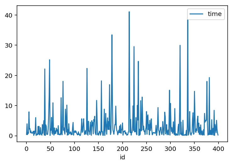
train.corr()With the above code, we can see the correlation with each feature and time. This result shows weak correlations with each feature and time. It means I need to work on feature engineering (feature selection). According to the above document, its complexity is
The major advantage of SGD is its efficiency, which is basically linear in the number of training examples. If X is a matrix of size (n, p) training has a cost of O(knp¯), where k is the number of iterations (epochs) and p¯ is the average number of non-zero attributes per sample.
Recent theoretical results, however, show that the runtime to get some desired optimization accuracy does not increase as the training set size increases.
That means one of critical factorts to affect its performance is the number of objects (n) * iterations or epochs (k) in our dataset, rather than making them independent each other. Also, the feature (parameter) penalty has 4 categories (options); ‘none’, ‘l1’, ‘l2’, and ‘elasticnet’. This should be handled as a categorial feature unlike other 14 numerical features. Thus, I create a function to create new feature, complexity like below to see correlation my new created feature and time.
def penalty_preprocessing(df, v):
'''
creates new feature 'complexity' according to the penalty option, v.
'''
new_df = df.loc[df['penalty'] == v]
new_df.loc[new_df['n_jobs'] == -1, ['n_jobs']] = 16
new_df.loc[:, ('complexity')] = new_df['n_samples'] * new_df['max_iter'] * new_df['n_features']
new_df.loc[:, ('complexity')] = new_df['complexity'] * new_df['n_classes']
new_df.loc[:, ('complexity')] = new_df['complexity'] / new_df['n_jobs']
new_df.loc[:, ('complexity')] = new_df['complexity'] + new_df['flip_y'] + new_df['random_state']
return new_df.loc[:, ('id', 'complexity', 'time')] For the complexity, max_iter represents k in the document, and n_samples * n_features * n_classes means overall the dataset’s matrix size np¯, which I mutiply them all. On the other hand, n_jobs makes the performance faster as it is the number of CPU. It should be devided the complexity, then. The maximum n_jobs in dataset is 16 in the training dataset, so I replace -1 which means using all jobs with 16.
penalty_none = penalty_preprocessing(train, 'none')
penalty_l1 = penalty_preprocessing(train, 'l1')
penalty_l2 = penalty_preprocessing(train, 'l2')
penalty_elasticnet = penalty_preprocessing(train, 'elasticnet')
The above code creates new dataframe for each penalty respectively. Now, I can see my new created feature ‘complexity’ is correlated with time more than 97% for every penalty option like below.
penalty_none.corr()| Tables | complexity | time | |
|---|---|---|---|
| id | 1.00000 | 0.032260 | 0.035770 |
| complexity | 0.03226 | 1.00000 | 0.980792 |
| time | 0.03577 | 0.980792 | 1.000000 |
penalty_l1.corr()| Tables | complexity | time | |
|---|---|---|---|
| id | 1.00000 | 0.057691 | 0.059486 |
| complexity | 0.057691 | 1.00000 | 0.988946 |
| time | 0.059486 | 0.988946 | 1.000000 |
penalty_l2.corr()| Tables | complexity | time | |
|---|---|---|---|
| id | 1.00000 | 0.064950 | 0.015912 |
| complexity | 0.064950 | 1.00000 | 0.982053 |
| time | 0.015912 | 0.982053 | 1.000000 |
penalty_elasticnet.corr()| Tables | complexity | time | |
|---|---|---|---|
| id | 1.00000 | 0.011534 | 0.025684 |
| complexity | 0.011534 | 1.00000 | 0.976314 |
| time | 0.025684 | 0.976314 | 1.000000 |
You can check all code here Google Colab Data Analysis link Click!
2.2 Feature engineering and Prediction
I should do feature engineering according to the above data analysis result. In this part, I use one-hot encoding to deal with the cetegorial feature, penalty and build a simple feed forward neural network with PyTorch for prediction.
2.2.1. Feature Scaling
I try normalisation and standardisation for rescaling data or __feature scaling __because of features which are highly varying in magnitudes, units and range.
def standardization(df):
'''
Z-score standardise
'''
quant_features = [n for n in df.columns[:-4]]
# Store scalings in a dictionary so we can convert back later
scaled_features = {}
for each in quant_features:
mean, std = df[each].mean(), df[each].std()
scaled_features[each] = [mean, std]
df.loc[:, each] = (df[each] - mean)/std
return df, scaled_features
def standardization2(df):
'''
normalisation
'''
quant_features = [n for n in df.columns[:-4]]
# Store scalings in a dictionary so we can convert back later
scaled_features = {}
for each in quant_features:
min_, max_ = df[each].min(), df[each].max()
scaled_features[each] = [min_, max_]
df.loc[:, each] = (df[each] - min_)/(max_ - min_)
return df, scaled_features2.2.2. Validation and Model
I split train data into train and validation dataset for validation and build a simple feed forward NN like below.
# Build a feed-forward network
model = nn.Sequential(nn.Linear(len(train_features[0]), 100),
nn.ReLU(),
nn.Linear(100, 70),
nn.ReLU(),
nn.Linear(70, 20),
nn.ReLU(),
nn.Linear(20, 1),
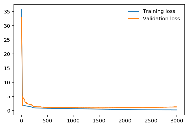
)The following plot is about training loss and validation loss per epoch.
My prediction result with validation data is like that:
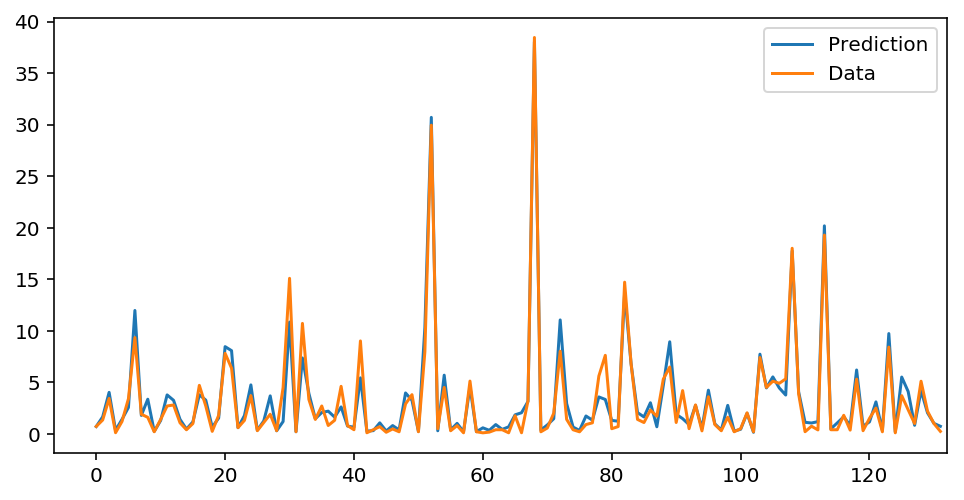
You can check all code here Google Colab Prediction with PyTorch link Click!
3. Future Work
- Replace n_jobs = -1 should be more sophisticated, not just 16, which requires another data anaysis task.
- Use scikit-learn to split train validation dataset, which is fancy, instead of Numpy array slicing.